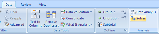
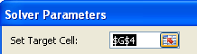
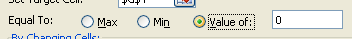
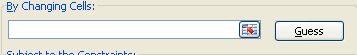
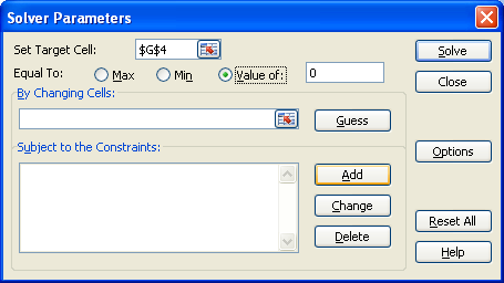
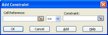
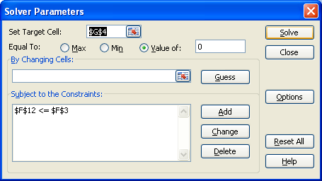
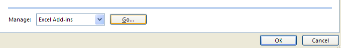
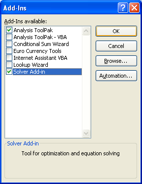
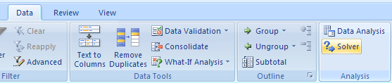
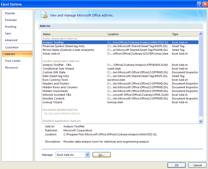
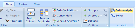
Use Solver

Click the Data tab. Then click the Solver button.

Select the target cell.

Click an Equal To option, and then, if necessary, enter a value.

Select the cell range the solver uses to compare against the target cell.

Click Add.

Enter specific cell reference and constraint, and then click Add.            Click OK.

Click Solve.

If the Solver finds a solution, the Solver Results dialog box opens.            Click the Keep Solver Solution option.            Click a report type.            Then click OK.

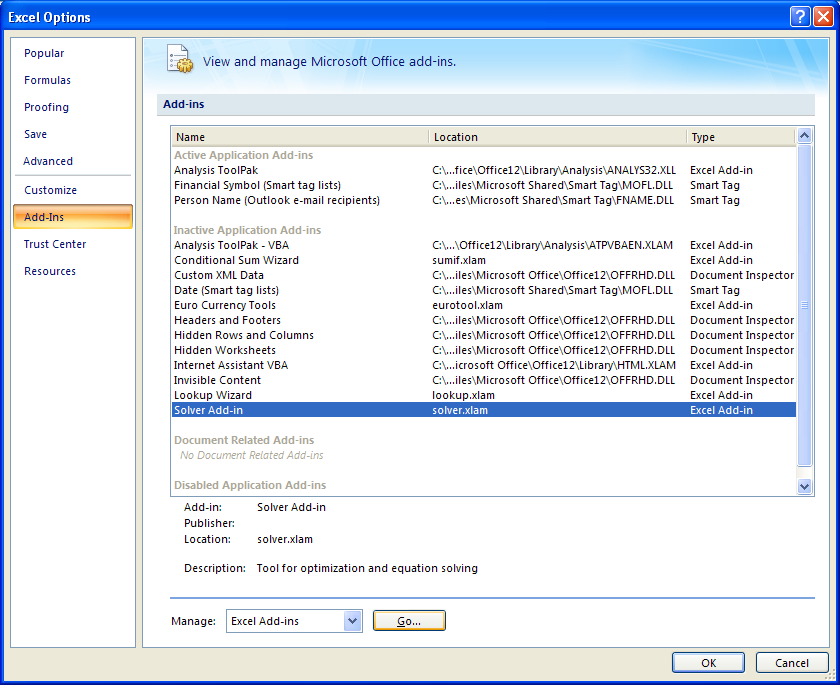
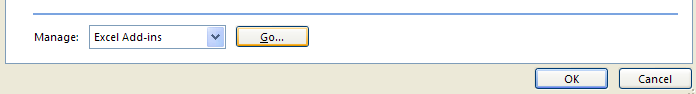
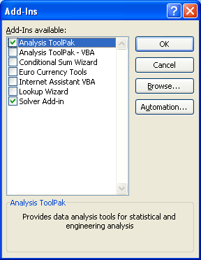
Add/Install Solver Add-in

Click office button. Then click the Excel Option.

Click the Add-in and click the solver in the list.

Click GO

Select Solver add-in in the list. Click OK.

Click OK to install Solver. Solver button is added to Data tab.

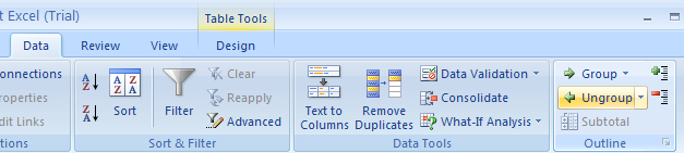
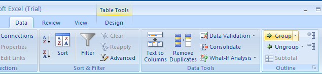
Clear an outline

Select the outline. Click the Data tab,
click the Group button arrow, and then click Clear Outline

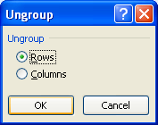
Ungroup outline data

Select the data group.  Click the Data tab and click the Ungroup button  arrow, and then click Ungroup.

Click the Rows or Columns option, and then click OK.

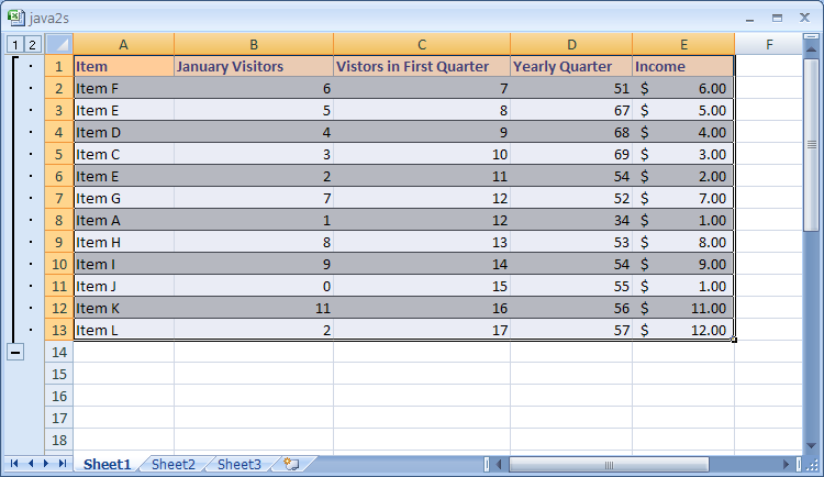
Create an Outline

Select the data.             Click the Data tab.            Then click the Group button arrow.             Then click AutoOutline.

Click a plus sign to expand an outline level;  click a minus sign to collapse an outline level

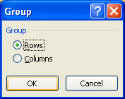
Create a Group

Select the data.  Click the Data tab and click the Group button arrow, and then click Group.

Click the Rows or Columns option.

Click OK.

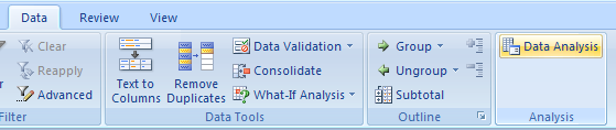
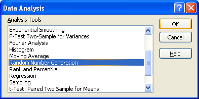
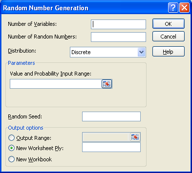
Use Data Analysis Tools

Click the Data tab.             Click the Data Analysis button.             If not available, load the add-in.

Click the analysis tool.

To get help about each tool, click Help.

Click OK.

Select the input range.  You can use the Collapse Dialog button to select  a range and the Expand Dialog button to return. Select the output range.  You can use the Collapse Dialog button to select  a range and the Expand Dialog button to return. Specify any additional tool-specific options. Then Click OK.

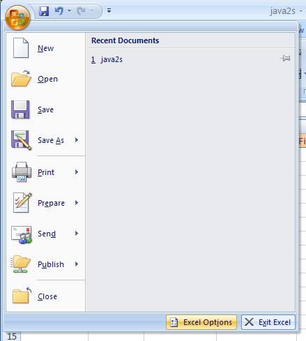
Add/Install Data Analysis Add-in

Click office button. Then click the Excel Option.

Click the Add-in and click the Data Analysis in the list.

Click GO

Select Data Analysis add-in in the list. Click OK.

Click OK to install Data Analysis.             And Data Analysis button is added to Data tab.

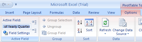
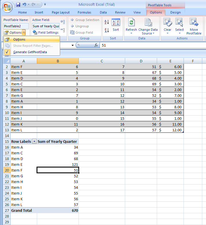
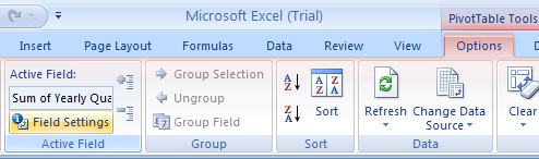
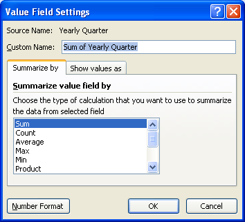
Rename a field in a PivotTable

Click the PivotTable report.             Click the Options tab.             Click the Active Field Name box,             type a new name and then press Enter.

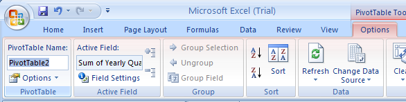
Rename a PivotTable

Click the PivotTable report.             Click the Options tab.             Click the PivotTable Name box and type a new name and then press Enter

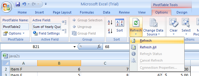
Refresh PivotTable

Click the PivotTable report.  Click the Options tab and then click the Refresh button

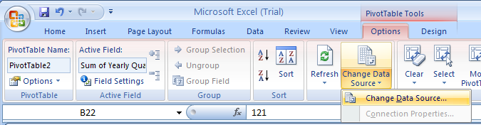
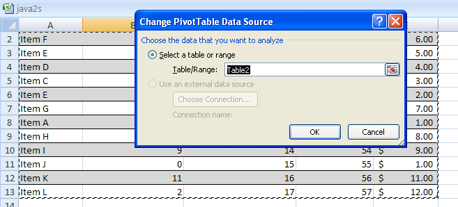
Select a different data source for a PivotTable

Click the PivotTable report.             Click the Options tab.             Click the Change Data Source button

Click the Select a table or range option,  or click the Use an external data source and specify a connection.

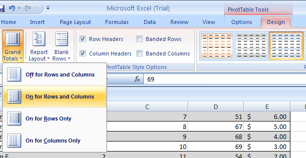
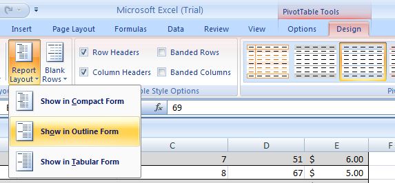
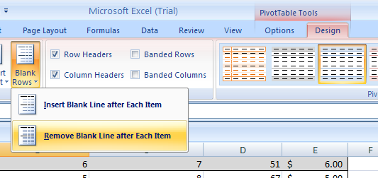
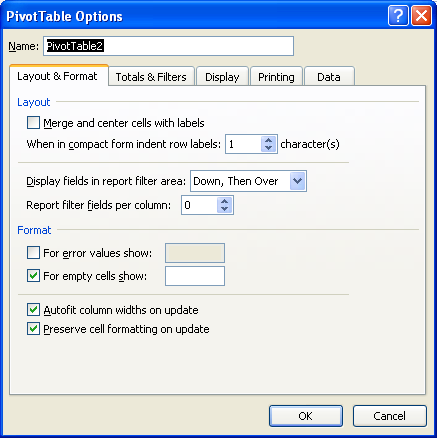
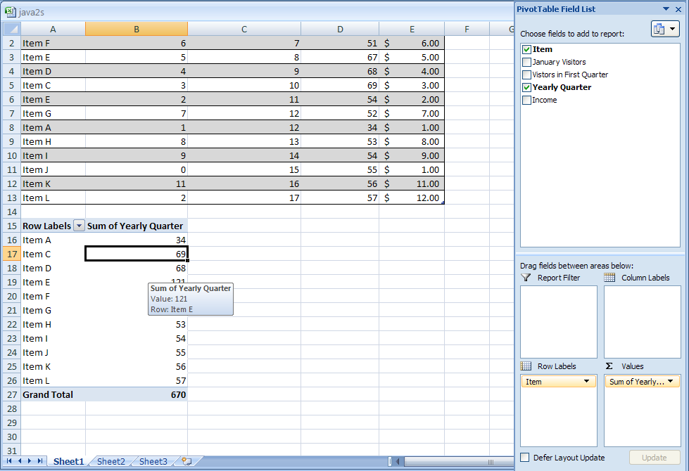
Format a PivotTable Report

Click any field in the PivotTable report.  Click the Design tab under PivotTable Tools.  Click the More list arrow under PivotTable Styles  and then click the PivotTable style.

Select or clear the PivotTable format options:  Row Headers, Column Headers, Banded Rows, Banded Columns.

Select Subtotals to show or hide subtotals.

Select Grand Totals to turn on or off grand totals for columns or rows.

Select Report Layout to set to compact, outline, or tabular form.

Select Blank Row to insert or remove a blank line after each item.

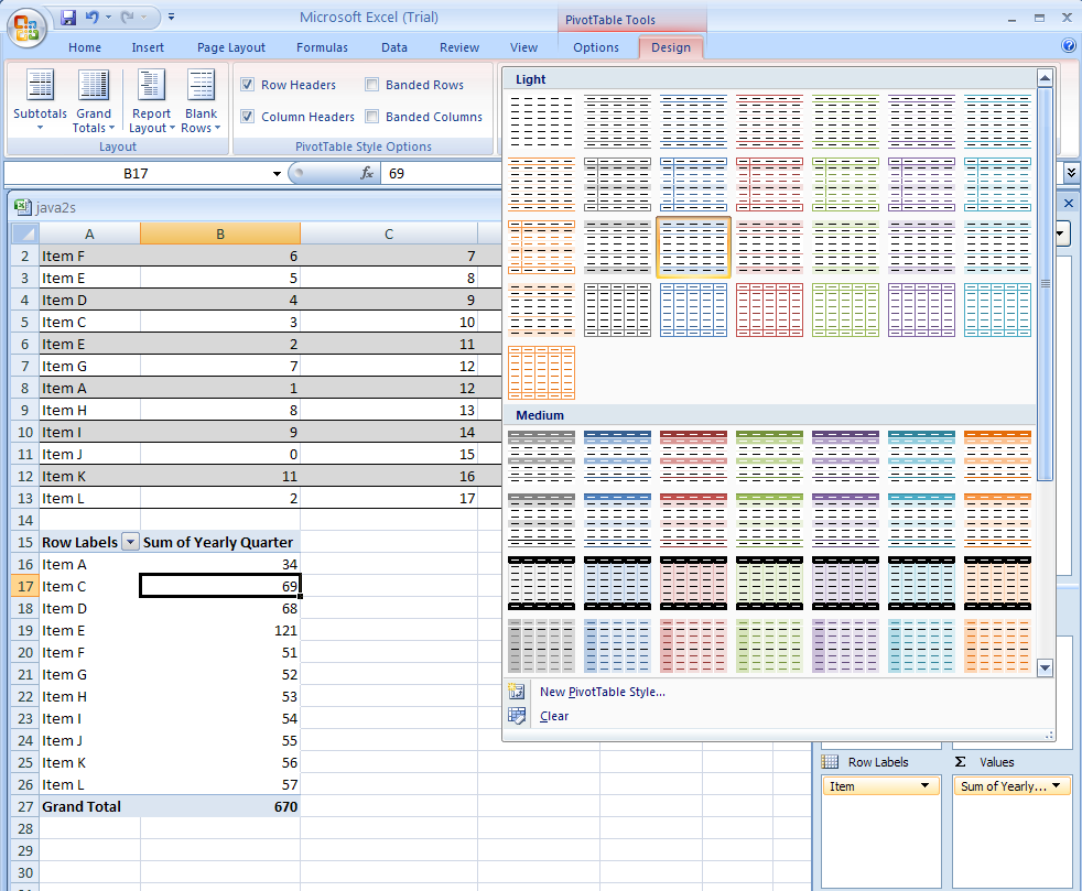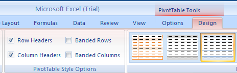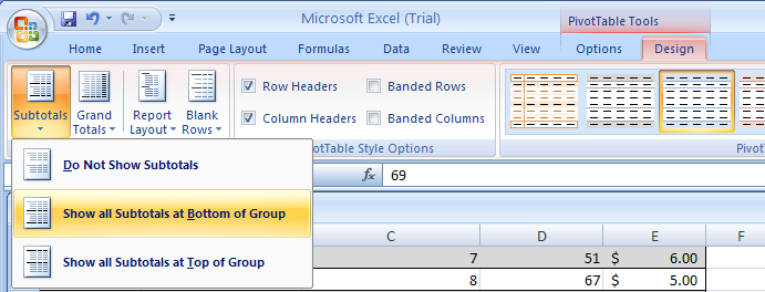
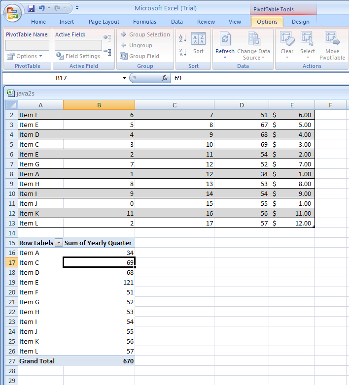
Modify a PivotTable Report

Click any field in the PivotTable report.             Click the Options tab under PivotTable Tools.

To change PivotTable options, click the Options button

Make the changes and then click OK.

To change field settings, select the field,             click the Field Settings button

Then Make the changes and then click OK.

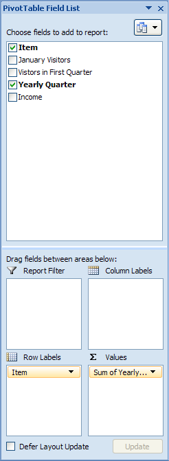
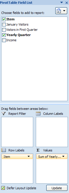
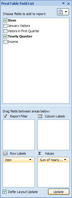
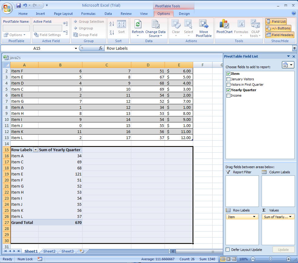
Add or Remove a Field in a PivotTable or PivotChart Report

Click any field in the PivotTable report.  Select/clear the check boxes next to the  fields you want to include or exclude  from the PivotTable and PivotChart.

To change the position of a field, drag the field in the Field list to: Values to display summary numeric data. Row Labels to display fields as rows on the side of the report. Axis field in a PivotChart. Column Labels to display fields as columns at the top of the report.  Legend field in a PivotChart. Report Filter to filter the entire report based on the selected  item in the report filter.

To enable manual layout updating, select the  Defer layout update check box.

Click Update to manually update the report layout.

Delete a PivotTable

Click the PivotTable report.             Click the Options tab.             Click the Select button.             Click Entire PivotTable. Then press Delete.

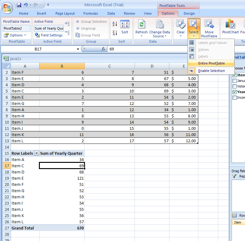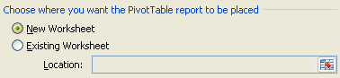
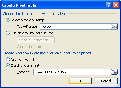
Create a PivotTable or PivotChart Report

Click anywhere within the table range.  Click the Insert tab.  Click the PivotTable button arrow and then click PivotTable, or PivotChart.

Click the Select a table or range option,  or click the Use an external data source option,  click Choose Connection, and then select a connection.

Click the New worksheet option or Existing worksheet option,             and specify a cell range.

Click OK.

Select the check boxes next to the fields you  want to use to add them to the empty PivotTable.