Conditional Formatting: Format Cell Contents Based on Ranking and Average

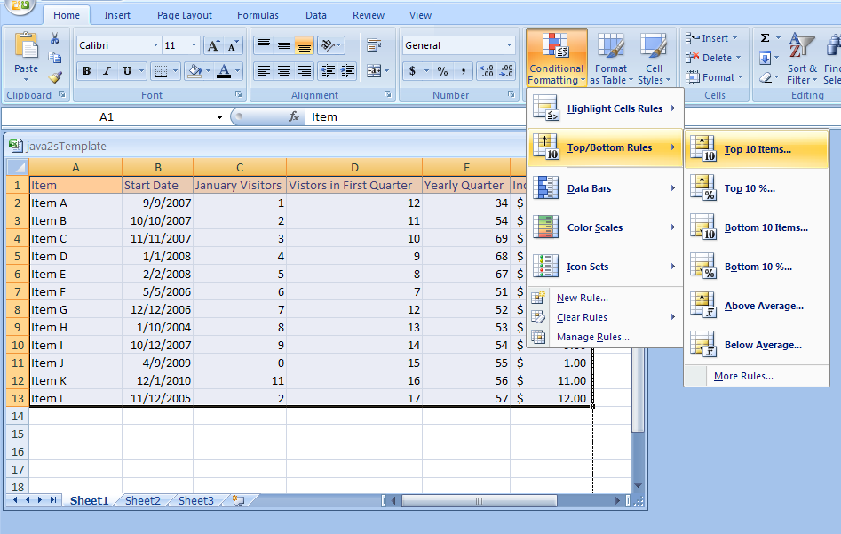
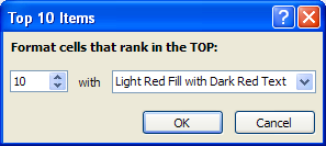
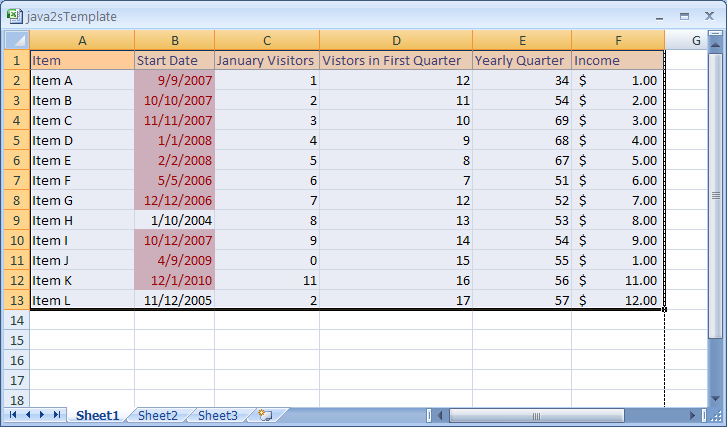
Select a cell or a range.  Click the Home tab.  Click the Conditional Formatting button.  Point to Top/Bottom Rules.  Click the comparison rule: Top 10 Items, Top 10 %, Bottom 10 Items, Bottom 10 %, Above Average, Below Average

Specify the criteria. Click OK.

Check the result.